
I found a great article on statistics by Scott Bradley Brixen of ListReports called “Reading Real Estate Statistics”. This might be tedious for some, but it you tend to geek-out over numbers like I do, you’re welcome and happy reading!
” Part 1: Better than Average
As you read through news stories and social media posts about residential real estate, you’re going to come across the average and median all the time. You probably know that the median is generally the preferable measure — but do you remember why? And even if you’re using the median, are you aware that it can have problems too?
This is the first in a series of articles designed to help you better understand (and assess the validity of) the real estate statistics you consume daily.
First, some definitions. If you know these already, skip to ‘Can the Mean and Median be the Same?’.
Average (or Mean):
Add up all the observations and divide by the number of observations. This is the simple average that we learned how to calculate in elementary school.
Observations: 2, 4, 7, 12, 13
Number of Observations: 5
Average: 7.6 [(2+4+7+12+13)/5]
Advantage: Easy to calculate.
Disadvantage: Can be skewed by ‘extreme’ observations.
Median:
The mean is the ‘middle’ observation; half of the observations are above it; half of them are below it.
If the number of observations is odd (let’s say 5), then the 3rd observation is your median.
If the number of observations is even (let’s say 6), then the median is halfway between the 3rd and the 4th observation.
- Odd number of observations: 2, 4, 7, 12, 13 [7 is the median]
- Even number of observations: 2, 4, 7, 9, 12, 13 [8 is the median = halfway between 7 and 9]]
Advantage: Reduces the impact of ‘extreme’ observations.
Disadvantages: Not easy to figure out without a computer if you’ve got a lot of observations (because they need to be put in numerical order first).
Lesson 1: Can the Average and the Median be the Same?
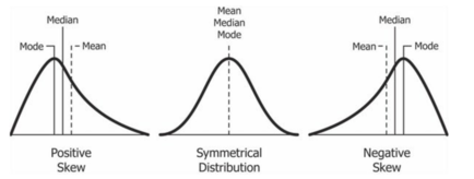
Sure they can. In a perfectly symmetrical distribution (like the middle ‘bell curve’ below), the mean and the median are the same. Unfortunately, few things in real estate are as perfectly distributed as this 🙂.
In a “positively skewed” distribution (like the curve on the left below), the average gets pulled to the right more than the median. Imagine that this is a graph of the prices of homes for sale. That long tail on the right could be a few, high-priced luxury listings.
In a “negatively skewed” distribution (like the curve on the right), the average gets pulled to the left more than the median. Perhaps that long tail on the left is the result of mistakenly adding in the price of plots of raw land into the analysis?
Lesson 2: Welcome to Echidna
Let’s consider the fictional New England town of Echidna. It’s a small place, with most of the people living in single family homes in the Wattawanka Valley. However, there are a small number of much higher-priced homes perched on the ridge that overlooks Echidna and the Wattawanka River. Currently, there are 20 homes for sale.
Table 1
Listing Prices in Echidna, New Shropshire
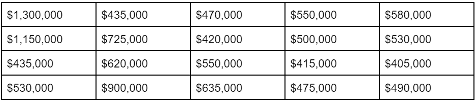
First, I’d like you to eyeball the listing prices. What do you think is the average?
You probably came up with a number close to $500,000. Here are the actual average and median.
Average: $605,750
Median: $530,000
There’s a big difference between the two! But why?
As you may recall from your local real estate coursework (or college statistics), the average can be skewed by ‘extreme’ observations, especially if the total number of observations is small.
So let’s remove the three luxury ‘high on the ridge’ listings ($1,300,000; $1,150,000; $900,000) and recalculate.
Table 2
Listing Prices in Echidna, New Shropshire [excluding luxury listings]
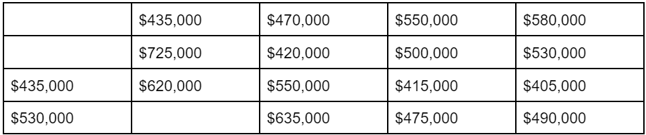
Average: $515,588
Median: $500,000
By removing those three luxury listings, the average drops by $95,000 but the median only drops by $30,000. The average and median are now fairly similar.
Note: Extreme observations can be on the low side too. Think about the impact that raw land or manufactured homes might have on your averages. If we replaced those three luxury listings with three raw land listings, look at what happens to the averages.
Table 3
Listing Prices in Echidna, New Shropshire [adding in 3 raw land listings]
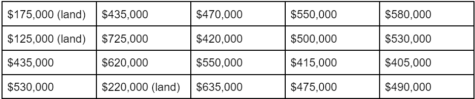
Average: $464,250
Median: $482,500
The gap between the average and the median has opened up again, but not as much as it did before. Why? Because the three luxury listings were $400,000-$800,000 above the median whereas the raw land listings were only $200,000-$300,000 below the median. In other words, the much higher-priced luxury listings pulled the average up more than the lower-priced raw land listings pulled the average down. Make sense?
Lesson 3: Apples and Oranges
The table below shows the listing prices of 10 homes in Laguna Beach, CA and 10 homes in Sheboygan, WI. Why would we combine these two very different places in the same dataset? To make a point.
In this example, neither the average nor the median are useful! The average of $1,449,000 is too low for Laguna Beach (only one listing is priced below it) and far too high for Sheboygan (four times the highest-priced listing). And the median, like it’s supposed to, is right in the middle. Unfortunately, right in the middle means a price that doesn’t exist in either Laguna Beach or Sheboygan!
Understanding what’s included in the sample is the first step to understanding how meaningful the median or average might be. In this example, the problem is that we’ve put apples and oranges in the same basket.
When you look at national real estate averages, New York State and California pull the national average and median listing price up. North Dakota and Louisiana pull it down. If you include or exclude certain states from a sample, you will end up with very different results — for the mean and the median! Same goes for statewide data if you include or exclude the capital or largest city!
Table 4
Listing Prices in Laguna Beach, CA and Sheboygan, WI
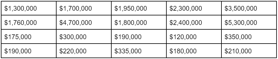
Average: $1,449,000
Median: $825,500
Lesson 4: Comparing Averages and Medians can be Messy
Everybody wants to know how much home prices are rising in their area. Let’s pretend that you’re an agent in Redding, CA. You go to realtor.com and find the median listing price today ($400,000) and one year ago ($420,000). You then calculate that home prices have fallen 5% in the last year.
But have they really?
Remember, you’re looking at the median price of homes that were on the market at a certain time. The homes that were on the market a year ago aren’t the same homes on the market today (I hope). What if a year ago, there were many more million-dollar listings as people ‘shot for the moon’ with their list prices. Whereas today, what the market really wants is homes under $500,000, and so you see many more ‘affordable’ homes listed.
This is known as the ‘mix’ issue. If the mix of high-priced/low-priced properties stays roughly the same, then you can compare averages and medians from different time periods. But if the mix changes, the comparison can be skewed and becomes less instructive.
In fact, it’s possible that home prices could be RISING across the board by 5%, but the average and median could be falling because there are a greater number of low-priced properties currently listed.
Note: If you really want accurate data on home price appreciation, you’re better off using numbers from Case-Shiller or the FHFA. Both indices use the ‘repeat sales’ method, where the last two transactions for the same home are the building blocks of the index.
Lesson 5: Other Things to Know
- The larger the sample size (i.e., the more observations), the less of an impact that a few extreme (really high or really low) observations will make on the average. That means that the difference between the average and median will likely decrease.
- But when the sample size decreases (like is happening with active inventory right now), the potential impact of extreme observations rises. The difference between the average and median will likely increase.
- You can’t add averages together. (Well, I guess you can, but mathematically it isn’t correct.) Instead, you can add ALL the observations together and then take the average of the larger dataset.
Final Reminder: Understanding what’s included in the sample is the first step to understanding how meaningful the median or average might be. Are luxury listings skewing the average higher? Are raw land listings skewing it down? Are you comparing apples and oranges? Could a shift in mix be an issue? “
Source: https://blog.listreports.com/reading-real-estate-statistics-fb5d5ca87cc3